Implementation notes of a CPU ray tracer

An implementation walkthrough of a CPU path tracer, from recursive ray scattering and polymorphic scene design to BVH acceleration and final renderings.

Final Renderings

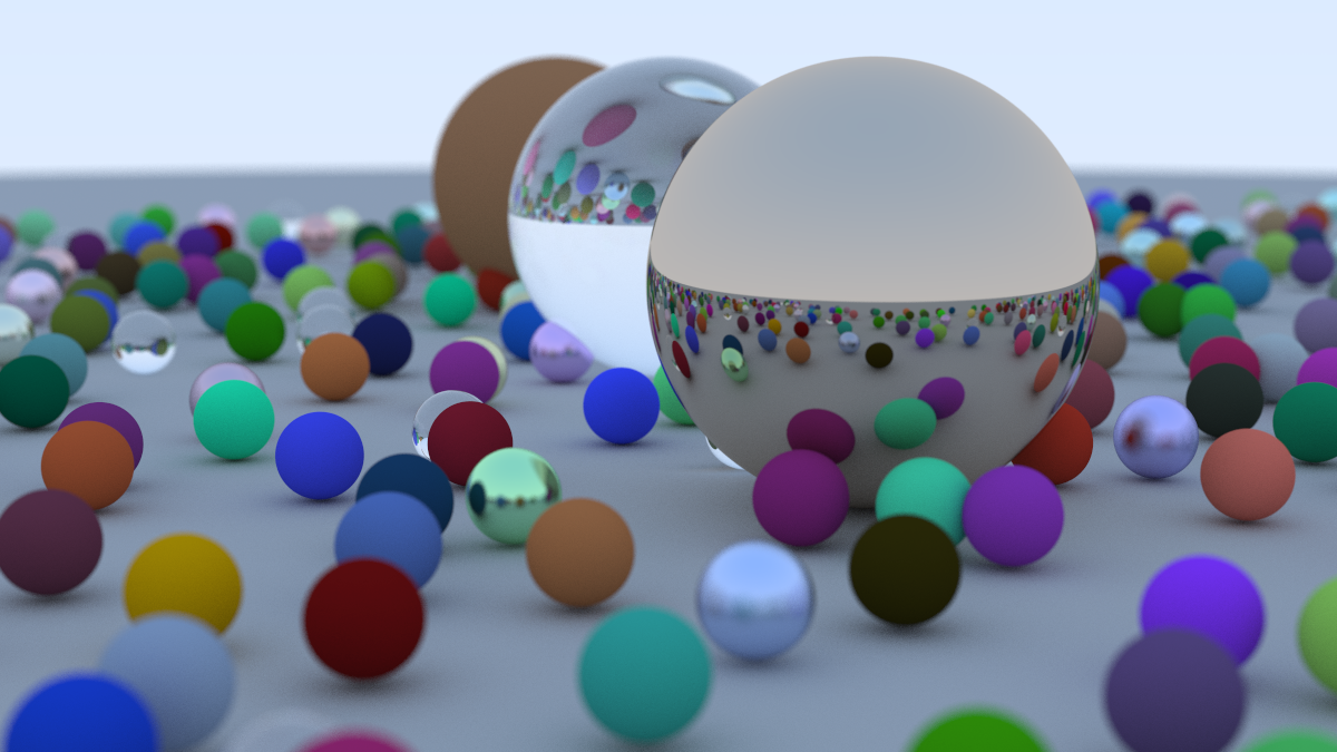
Random Sphere Scene

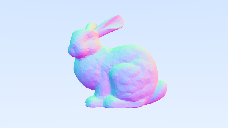
Stanford Bunny

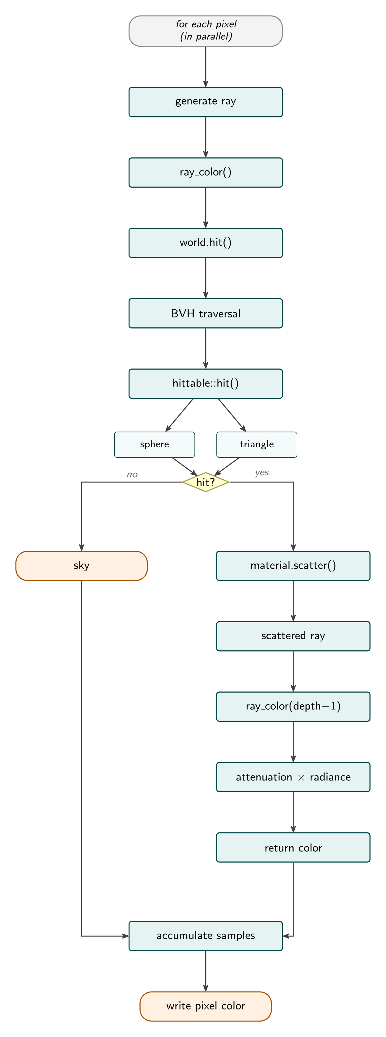
Architecture Overview

Core Components

The renderer is built upon a list of abstractions that separate ray generation, geometry represenation, material interaction, and acceleration structure.

Component	Role	Entry Point
camera	Generates rays and drives the parallel render loop	render(world)
hittable	Abstract base for anything a ray can intersect	hit(), bounding_box()
Sphere, triangle	Concrete geometric implementation of hittable	—
hittable_list	Holds the scene’s objects; is a hittable	hit()
material	Abstract base for surface response	scatter()
lambertian, metal, dielectric	Diffuse, reflective, and refractive surfaces implementation	—
bvh_node, aabb	Bounding-volume hierarchy for fast intersection	hit()
vec3, Ray, color	Math primitives	—

---

Rendering equation

color camera::ray_color(const Ray &r, const hittable &world, int depth)
{
    hit_record rec;
    if (depth == 0)
    {
        return color(0, 0, 0);
    }
    if (world.hit(r, 0.001, infinity, rec)) //returns true if the ray hits an object
    {
        Ray scattered;
        color attenuation;
        
        if (rec.mat->scatter(r, rec, attenuation, scattered))
        {
            return attenuation * ray_color(scattered, world, depth - 1);
        }
        return color(0, 0, 0); //if the scatter function of the material returns false, return black
    }
    // sky:the default color of a ray, when it doesn't hit anything
    vec3 unit_dir = unit_vector(r.direction);
    double a = 0.5 * (unit_dir.y() + 1.0);
    return (1.0 - a) * color(1.0, 1.0, 1.0) + a * color(0.5, 0.7, 1.0);
}

When a ray hits a material and scatters:

$$
L_o = T \cdot L_i
$$

Where:

• $L_o$: outgoing radiance
• $L_i$: incoming radiance
• $T$: attenuation (material reflectance)

Here, a recursive structure is used. In particular, the equation is the attenuation (put simply, a property of the material acting as an RGB “filter” on a ray) multiplied by the color of the scattered ray. As we learned in junior high physics, the “color” of an object is created due to the reflection of sunlight, and since the ray path is invertible, we can also trace it using this model.

Polymorphism of hittable and materials

Definition: Polymorphism allows a base-class pointer to refer to an object of any derived type, so that the same function call automatically will lead to different behavior at runtime, depending on the actual type of the object being referred to.

Here are a few examples of polymorphism in the ray tracer

if (world.hit(r, 0.001, infinity, rec))   // world's class is hittable list 

And the hit function of world itself has the following form

// hittable_list::hit
for (const auto &obj : objects) {
    if (obj->hit(r, t_min, closest_t, temp)) { ... }   // obj has the type of shared_ptr<hittable>
}

Specifically, obj->hit(r, t_min, closest_t, temp) runs different code depending on what obj actually is at runtime: a bvh_node, Sphere, or triangle, though the call site only ever sees the hittable interface.

Another example is about the scattering of materials

if (rec.mat->scatter(r, rec, attenuation, scattered))   // rec.mat has the type of shared_ptr<material>

And the specific material implementations (i.e. lambertian, metal, and dielectric) are implemented in material.h.

BVH acceleration

In the old version where we don’t have the BVH, the call world.hit (hittable_list::hit) traverses every object in the scene:

for (const auto &obj : objects) {   // objects[0], objects[1], ... object[n] are all tested
    if (obj->hit(r, t_min, closest_t, temp)) { ... }
}

This costs O(N) per ray, and the loop must check every object to make sure no closer one exists. This is far too slow for a mesh like the Stanford Bunny with tens of thousands of triangles.

With the bounding volume hierarchy (BVH), the scene is organized into a binary tree of axis-aligned bounding boxes (AABBs). If a ray misses a node’s box, then every triangle or sphere inside that box is excluded at once — the whole subtree is skipped. As a result, each ray only tests the regions it actually passes through:

bool hit_left  = left->hit(r, t_min, t_max, rec);
bool hit_right = right->hit(r, t_min, hit_left ? rec.t : t_max, rec);
return hit_left || hit_right;

Two things happen here. First, both children are tested, because a single ray can pass through both boxes; it keeps traversing until it reaches the leaves and finds the closest hit. Second, note the hit_left ? rec.t : t_max in the right call: once the left side has a hit, the right side is searched only for something closer than that hit, by reducing t_max to rec.t. This keeps rec holding the nearest intersection and prunes away farther boxes for free.

Overall, instead of testing all N objects, a ray walks down the tree, rejecting whole subtrees with cheap box tests and doing real triangle intersection only in the few leaves it reaches — bringing the per-ray cost from O(N) down to roughly O(log N).